EXERCISE 9: OBJECT TRACKING

This exercise is about object tracking, wherein we need to locate a moving object in a video.

To implement object tracking, we did the same approach with background substitution exercise. First we convert our input video to grayscale. We set the first frame as the background model. We then compute the difference between the model and the next frames, and convert the video to binary.

After binarizing the video, we detected the object’s path. We checked the frames pixel by pixel if it is a background or a foreground. If it is foreground, we colored the output image white. So that for every frame, every foreground will be white (object’s path).

Here is the link for our input video: https://youtu.be/bJmTfabYb_U

And here is the output image for the path of the object

EXERCISE 7: CHROMA KEYING

The exercise this week is about chroma keying, wherein we need to change the background of a green screen video to our desired background.

To implement chroma keying:

1. Read two videos: the green screen video and the video with our desired background.
2. Convert the color space of the green screen video to HSV color space (for easier background detection)
3. Detect the green background from the green screen video.
4. Use morphological functions like erosion and dilation to lessen the image noise.
5. Detect pixel by pixel of the frame if it is a background or a foreground:
   • if background; change the values of the bgr of the background to the bgr values of the desired background to be overlayed.

*: The videos used for this exercise were downloaded from Youtube.

Here are the snapshots of the video inputs and output:

forevid

backvid

out

EXERCISE 10: AUGMENTED REALITY

For this exercise, a code was provided  but it only allows of overlaying a certain input image onto a pattern (chessboard pattern). It doesn’t have a sense of orientation, when the pattern moves or rotates nothing happens to the input image that is overlay-ed. So for our exercise we were asked to modify the code so that it will have a sense of orientation, such as if the pattern is rotated the image that is overlay-ed will also rotate along with it.

In order to do this we need two points to compute for the angle of rotation. To compute for the angle of rotation we used the formula:

angle = atan2(vector2.y – vector1.y, vector2.x – vector1.x)

and since the output of that is not in degrees we multiplied the answer to:

deg = ((angle) * 180) / 3.14159265

After doing this we used the builtin function in OpenCV for computing the rotation matrix: getRotationMatrix2D()

After computing the rotation matrix, the warpAffine() function is applied to rotate the image to its new points.

Here are the sample output:

1

2

3

4

5

Exercise 4: Connected Components

For this exercise we need to implement the Connected Components Algorithm, to detect the objects in an image.

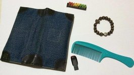
The input image that we used in this exercise contains 5 different objects:

First, we converted the image to a gray scale image and then applied the blur() and medianBlur() to produce a smoother image. Then a threshold() function was applied to convert the grayscale image to a binary image.

After this, we applied the connected components algorithm.

For the connected components, a 2×2 integer array was created and contains 0 as initial values. The algorithm has two passes, for the first pass the image is traversed to check if the pixels is a foreground or a background, in this pass only the black pixels or pixels with a 0 value will be considered. So for each black pixel we check for its top and left neighbors, if the label in the arrlbl of the neighbors is 0.

• If both the top and left pixels are labelled 0, a new label will be created and will be added to the equivalence table.
• If only top pixel is labelled 0, we will copy the label from the left pixel.
• If only left pixel is labelled 0, we will copy the label from the top pixel.
• If both pixels are labelled 1, we will still copy the label from the top pixel; however, we will add the pixel with the larger label to the equivalent row of the smaller label.

For the second pass, the image will be traversed again, background pixels will not be considered. From the last label to the first label. From the equivalence table, higher values are converted to smaller ones based from their equivalence.

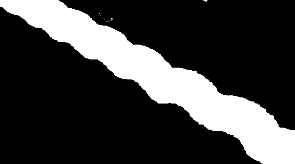
After applying the second pass, we now proceed to coloring the image according to their labels.  And this is the output of the labelled image:

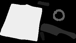
In order to use the rectangle() function to box the labels, we needed the upper-left and the lower-right vertex of each object and use it as parameters for the function. And this is the output image:

 

 

EXERCISE 8: BACKGROUND SUBTRACTION

For this exercise we need to use background subtraction in order to differentiate the foreground from the background.

The method that we used to be able to implement background subtraction is frame differencing wherein:

1. Take the frame (preferably the first where there are no objects yet or it is empty) and set this as the background model.
2. Then each succeeding frames is compared to the background that was set.
3. Then the next frames will be considered as the next background model.

With the use of the function absdiff() the difference between the background models and the gray scale frames (images) where determined. And the difference between these two is determined to be the foreground or the object that is moving.

After determining the foreground, the foreground image is converted to a binary using the threshold() function.

The input video will be sent to our instructor and the output of the will be shown when the code is executed.

Here are  sample images of the input video and the output of the Background Subtraction:

Input

Output

EXERCISE 6: PSEUDO COLOR IMAGE PROCESSING

PSEUDO COLOR IMAGE PROCESSING

For this exercise we were asked by our professor to apply on a weather map a pseudo color and use intensity slicing. To identify or detect the storms in the map.
To detect the storms the concept of intensity slicing should be implied. In intensity slicing specific range of intensities are being highlighted.

For our implementation of the exercise, the image is first converted to a gray scale image then pseudo coloring was applied. We set a threshold of 195 (we selected this value because for us it detects the storms accurately than other values) , meaning intensities that are greater than 195 are being highlighted and the colors of the gray intensities were changed according to the color gradient from the colors.jpg image and intensities that are 195 and below will not change (same color as the input image will be used for the output). The color palette was resized to a size of 1 x 255 so new values of the pixels would be identified easily.

if(src_gray.at<uchar>(i,j) > 195){
dst.at<Vec3b>(i,j) = resizedpalette.at<Vec3b>(0, src_gray.at<uchar>(i,j));
}
else{
dst.at<Vec3b>(i,j) = src.at<Vec3b>(i,j);
}

The input, color palette and output images are shown below.

colors.jpg

map.jpg

output.jpg

My partner, Yla Bandian and I did the exercise together. There are no separate contributions to the exer because we both thought on how to implement the exercise and experimented on the threshold values to set. 🙂

Exercise 3: Adaptive Thresholding

For this exercise, the task was to produce a binary image of a colored image. To do this we need to implement the adaptive threshold. Adaptive threshold may be computed by getting the mean of the 3×3 element structure that is slide from pixel to pixel, so each pixel will have a different threshold value.

To lessen the noise of the image, we first used the blur function on the image. After blurring the image, we computed for the mean and subtracted the value 5 so the noise would be lesser. The computed value will be the adaptive threshold then it would be compared to each pixel value of the image and if the pixel value is lesser than the threshold it will be classified as background (white) and if it is greater it would be classified as a foreground (black).

test.jpg

test_binary.jpg

 

 

CMSC 165 EXERCISE 2: FILTERING

For our 2nd exercise in CMSC 165 we were asked to implement our own spatial filtering and mean filtering without using the filter2d() function of OpenCV or any other function for filtering that is already provided by OpenCV. Me and my partner Yla Bandian separated the tasks she did the mean filtering part and I did the spatial filtering.

The upper image is the source image and the other consecutive images are the output images that we are able to obtain from the source image after implementing the spatial and mean filters. The two images at the bottom of the source image are the output images after applying the unweighted and weighted mean filters. And the bottom most images are the output images after applying the laplacian and sharpen spatial filters.

Source

Unweighted Output

Weighted Output

Laplacian Output

Sharpen Output

I was able to implement the laplacian spatial filter and sharpen spatial filter by using nested for loops the first two for loops is for accessing the pixel values of the image source and the other two consecutive for loops is for accessing the values inside the given kernel. The loops were nested to be able to perform an element wise multiplication of the pixel values and the values in the kernel and getting the total of the products. After getting the sum of the products, the values of a certain pixel will be changed to the value of the obtained sum, as for spatial filter the absolute value of the obtained sum will be used. The kernel containing the values [0, -1, 0, -1, 5, -1, 0, -1, 0] was used for the sharpen filter and the kernel with the values [0, 1, 0, 1, -4, 1, 0, 1, 0] was used for the laplacian filter.

CMSC 165 EXERCISE 1

Original Image

Output Image

Day Image ( Original and Output )

For the day image, comparing the two images the colors in the right picture (output
image) are more visible and the details of the fur near the dog collar can be seen
than in the original image. The colors were more emphasized and seen. To obtain this contrast I used the function:  return((0.003*channel*channel)-(0.023*channel));

Original Image

Output Image

Night Image ( Original and Output )

For the night image, if you compare the two images the cat in the right picture (output image) is more visible than in the original image. With the colors of the image being more emphasized in the output image more details about the picture were seen and has been visible. The color of the cat was also seen. So for me the contrast of the output image was just enough to be able to see more details about the picture. I used the function that is similar to the slope of line equation to obtain the output image; return(2*channel+3);